
50% Tech + 50% Energy: Does This Simple Portfolio Beat the S&P 500?
A viral tweet claims: just put 50% in Tech (XLK) and 50% in Energy (XLE) and you beat the S&P 500. We ran 22 years of data against it – with real transaction costs and different rebalancing frequencies. Spoiler: The thesis holds up – but not without caveats.
The Thesis
John Arnold posted a table on X showing the annual returns of XLK (Tech), XLE (Energy), and a 50/50 mix of both. His message: the combined portfolio delivers higher returns with a better Sharpe ratio than either sector alone. The reason: Tech and Energy often move in opposite directions – when one sector weakens, the other runs.
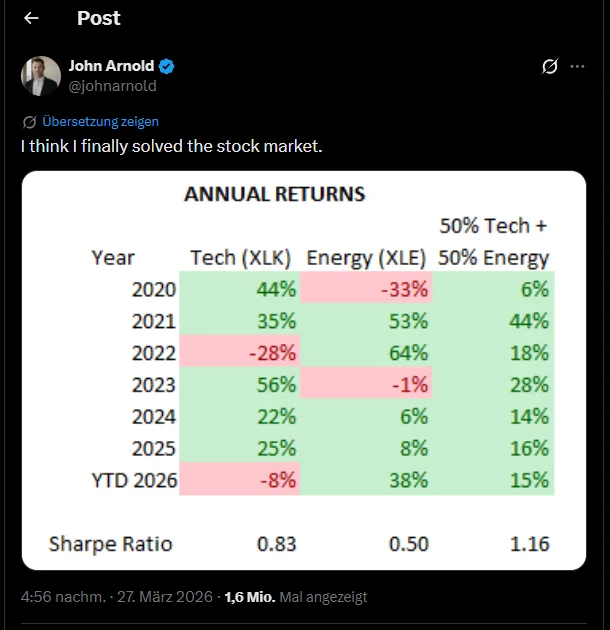
Sounds too simple to be true? We let the data speak – not just for the last few years, but over the entire common time frame since September 2003.
The Methodology
Period: 09/10/2003 to 04/14/2026 – 5,684 trading days (~22 years). Starting capital: $10,000, allocation 50% XLE / 50% XLK. Simulation: Share-based with fractional shares, no simplified weight approximation.
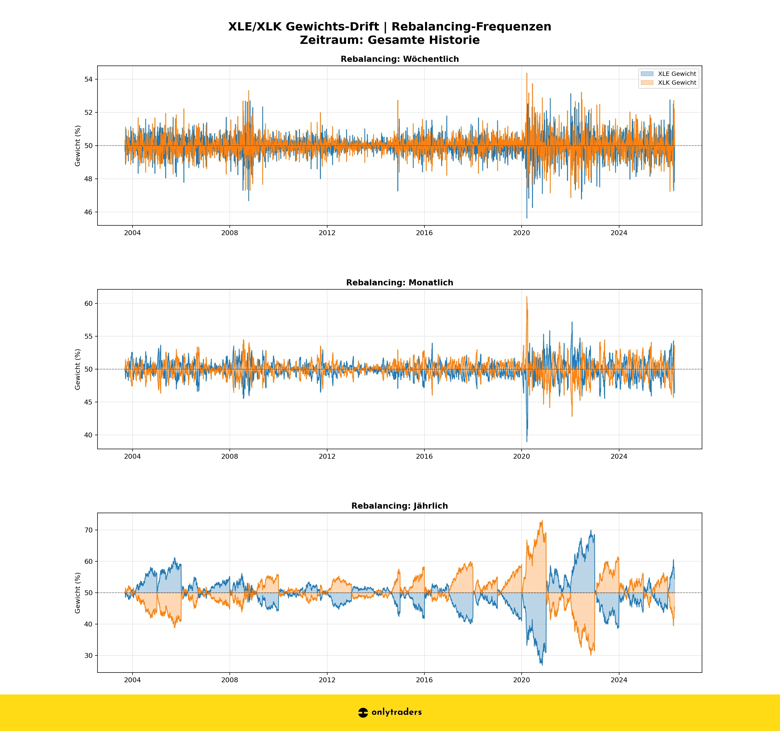
We test three rebalancing frequencies: weekly (1,180 events), monthly (272 events),
and yearly (24 events). Benchmark is SPY Buy & Hold. Transaction costs follow the
Interactive Brokers model: max(0.005 × shares, $1.00) per order – each rebalancing
triggers 2 orders (XLE + XLK).
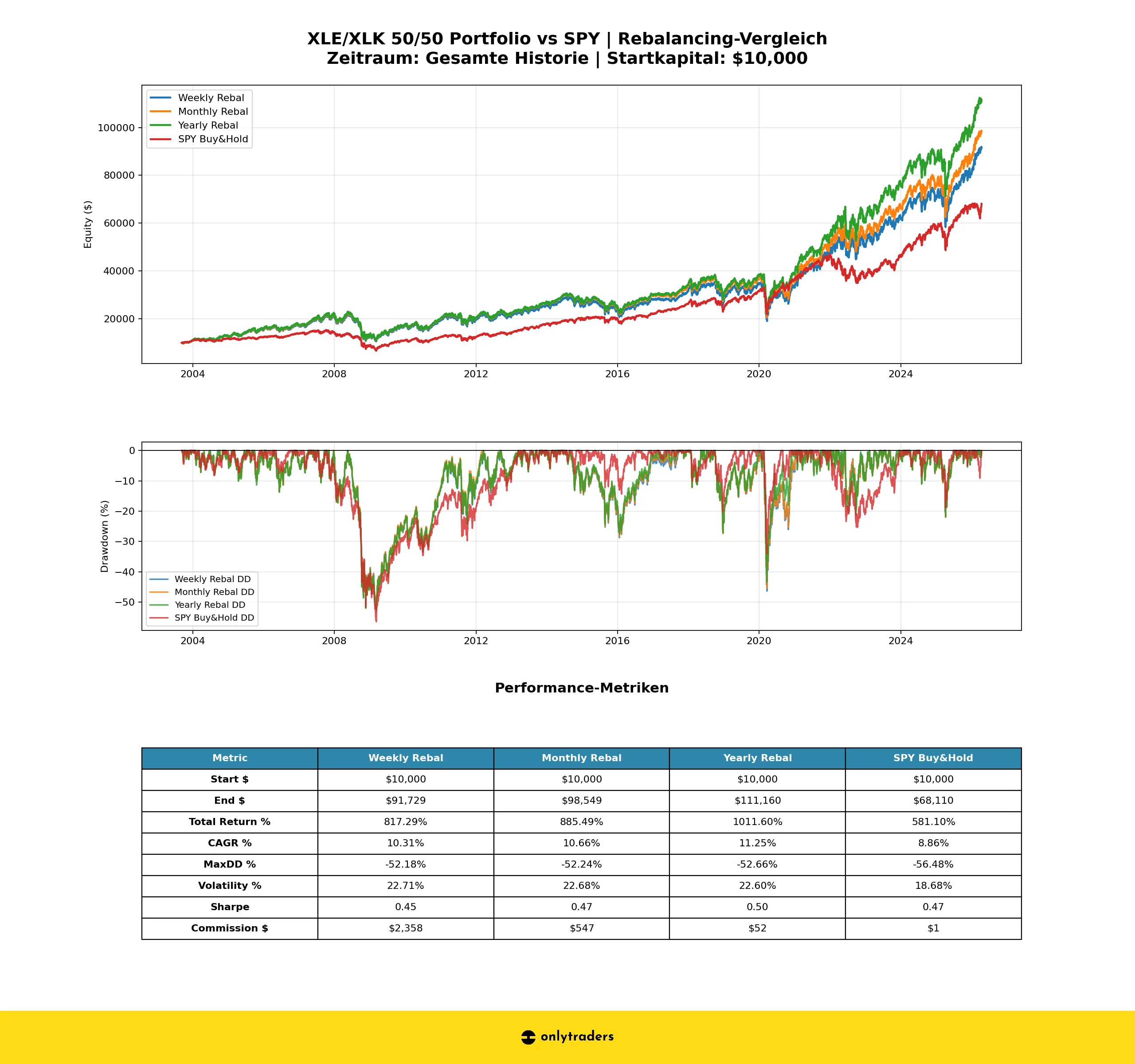
Results: Performance Without Transaction Costs
| Metric | Weekly | Monthly | Yearly | SPY B&H |
|---|---|---|---|---|
| Final capital | $101,519 | $100,814 | $111,399 | $68,111 |
| Total return | 915% | 908% | 1,014% | 581% |
| CAGR | 10.80% | 10.77% | 11.26% | 8.86% |
| Max drawdown | -51.90% | -52.17% | -52.65% | -56.47% |
| Volatility (ann.) | 22.71% | 22.68% | 22.59% | 18.68% |
| Sharpe ratio | 0.48 | 0.47 | 0.50 | 0.47 |
All three rebalancing variants clearly beat SPY: +1.91% to +2.40% CAGR per year. Yearly rebalancing delivers the highest return – rebalancing less often lets stronger trends run longer. The Sharpe ratio of the yearly portfolio (0.50) is better than SPY (0.47), despite higher volatility. And the MaxDD? ~52% for the portfolio vs. -56.5% for SPY.
And the Costs?
Theory is nice – but what’s left after fees? We calculate with the Interactive Brokers model.
| Variant | Total commission | Final capital loss | CAGR impact |
|---|---|---|---|
| Weekly rebal | $2,358 | -$9,790 | -0.50% |
| Monthly rebal | $547 | -$2,265 | -0.11% |
| Yearly rebal | $52 | -$239 | -0.01% |
| SPY Buy & Hold | $1 | -$1 | ~0.00% |
The result is clear: weekly rebalancing eats up almost $10,000 in final capital through 1,180 rebalancing events. Yearly rebalancing costs just $52 over 22 years – effectively irrelevant. The outperformance vs SPY remains at +2.39% CAGR after fees for yearly rebalancing.
Yearly Performance: 24 Years in Detail
| Year | Yearly rebal | SPY B&H | Delta |
|---|---|---|---|
| 2003 | 10.73% | 9.14% | +1.59% |
| 2004 | 17.48% | 8.67% | +8.81% |
| 2005 | 21.84% | 3.50% | +18.34% |
| 2006 | 10.20% | 11.78% | -1.58% |
| 2007 | 27.26% | 3.42% | +23.84% |
| 2008 | -40.46% | -37.74% | -2.72% |
| 2009 | 28.54% | 19.88% | +8.66% |
| 2010 | 12.15% | 10.96% | +1.19% |
| 2011 | 0.23% | -1.22% | +1.45% |
| 2012 | 6.15% | 11.70% | -5.55% |
| 2013 | 20.58% | 26.45% | -5.87% |
| 2014 | 3.78% | 12.37% | -8.59% |
| 2015 | -10.19% | -0.76% | -9.43% |
| 2016 | 19.66% | 11.20% | +8.46% |
| 2017 | 12.97% | 18.48% | -5.51% |
| 2018 | -13.09% | -7.01% | -6.08% |
| 2019 | 25.24% | 28.65% | -3.41% |
| 2020 | 0.89% | 15.09% | -14.20% |
| 2021 | 41.08% | 28.79% | +12.29% |
| 2022 | 11.88% | -19.95% | +31.83% |
| 2023 | 27.75% | 24.81% | +2.94% |
| 2024 | 12.57% | 24.00% | -11.43% |
| 2025 | 13.66% | 16.64% | -2.98% |
| 2026* | 12.54% | 1.65% | +10.89% |
*2026: Only until 04/14/2026 (partial year)
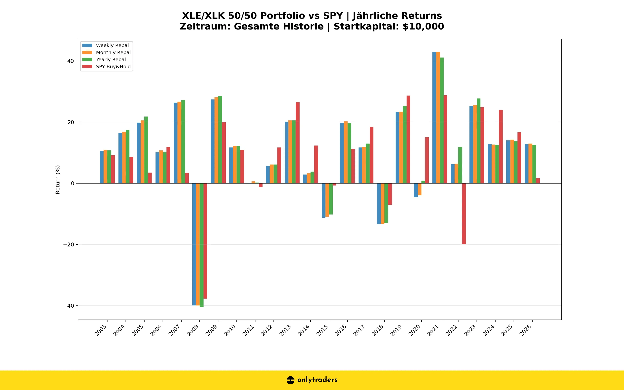
Outperformance Statistics
In 12 of 24 years, the portfolio beats SPY – exactly 50/50. But the distribution is asymmetric: in good years the portfolio wins by an average of +10.86%, in bad years it only loses -6.44% against SPY. The key year is 2022: while SPY drops almost 20%, the portfolio gains nearly 12% – a delta of over 31 percentage points.
Decade Analysis
| Decade | Portfolio (ann.) | SPY (ann.) | Difference |
|---|---|---|---|
| 2000s (2003–2009) | 7.89% | 0.83% | +7.06% |
| 2010s (2010–2019) | 7.03% | 10.53% | -3.50% |
| 2020s (2020–2026) | 16.60% | 11.76% | +4.84% |
Interpretation
2000s: The portfolio dominates massively. Energy benefited from the commodity supercycle, Tech hadn’t yet recovered from the dotcom crash. SPY suffered under the financial crisis – so did the portfolio, but the lead from 2004–2007 was big enough.
2010s: SPY clearly beats the portfolio. The FAANG rally drove the cap-weighted S&P 500, while Energy suffered under the shale oil oversupply and the oil price collapse 2014–2016. A pure XLK investment would have been better here.
2020s: Portfolio ahead again. Sector rotation after COVID: Energy benefited from the oil price surge 2021–2022, Tech stayed strong long-term. 2022 was the key moment – exactly the kind of regime in which this strategy shines.
Risk Profile: Drawdowns and Correlation
| Strategy | Max drawdown | Peak | Trough | Duration |
|---|---|---|---|---|
| Yearly rebal | -52.66% | 05/19/2008 | 03/09/2009 | ~10 mo. |
| SPY Buy & Hold | -56.48% | 10/09/2007 | 03/09/2009 | ~17 mo. |
Both strategies share the same trough – 03/09/2009, the bottom of the financial crisis. But the portfolio reached its peak only in May 2008, seven months after SPY. The reason: Energy was still rising while the overall market was already falling. The portfolio’s MaxDD is ~4% lower than SPY’s, but the annualized volatility at 22.6% is clearly higher than SPY’s 18.7%.
The daily return correlation between portfolio and SPY is 0.90 – high, but not perfect. The 10% decorrelation explains the diversification effects and the phases of strong outperformance.
Conclusion: The Thesis Holds – With Caveats
- Yes, the portfolio beats SPY: Over 22 years, the 50/50 XLE/XLK portfolio delivers a CAGR of 11.25% vs. 8.86% – a lead of +2.39% per year, after transaction costs.
- Yearly rebalancing is optimal: Just $52 total commission over 22 years. More frequent rebalancing destroys returns through costs and cuts off trends.
- The driver is sector rebalancing: Counter-cyclical shifting between two structurally negatively correlated sectors generates the edge. In crises like 2022 (SPY -20%, portfolio +12%), the effect shows most strongly.
- Outperformance is not constant: In the 2010s, SPY was ahead (+3.5% p.a.), driven by the tech mega-cap rally. The strategy needs regime-changing markets.
- Higher risk: Volatility is ~22.6% vs. ~18.7% for SPY. The better Sharpe ratio (0.50 vs. 0.47) only narrowly compensates.
Caveats
- Survivorship bias: XLE and XLK have existed since 1998/1999. The analysis starts in 2003 – the dotcom bubble is not included.
- Sector concentration: 100% in only 2 sectors is a concentration risk.
- Regime dependency: The strategy only works as long as Energy and Tech stay anti-correlated and both deliver positive returns long-term.
- No taxes: Every rebalancing triggers capital gains tax – not accounted for here.
- EU tradability: XLE and XLK are US-listed ETFs and cannot be directly traded by EU retail investors due to the missing PRIIPs KID. Anyone implementing the strategy in the EU has to switch to UCITS equivalents (e.g. SPDR S&P U.S. Energy / Technology Select Sector UCITS ETF). Their history is shorter, TER and tracking differ – the backtest would have to be re-validated with the UCITS variants.
So: John Arnold is right – but the strategy is no free lunch. It works because you systematically trim the winning sector and top up the loser. That requires discipline and the conviction that Energy and Tech will continue to have opposite cycles. For EU investors there’s an additional note: XLE/XLK aren’t directly tradable here – the next logical step would be a backtest with the UCITS equivalents to check whether the edge holds there. For those who believe that, this is a statistically robust approach.